New blog site
Hi
I am busy rewriting my blog posts to another blogging project.
Please find my newest and oldest posts on the new ZS1SCI site.
Have a wonderful day!
Cheers
Hi
I am busy rewriting my blog posts to another blogging project.
Please find my newest and oldest posts on the new ZS1SCI site.
Have a wonderful day!
Cheers
I recently purchased my first HF transceiver a Xiegu G90.
Since I would mostly just be interested in digital modes, Flrig seemed like the obvious choice to control the radio via CAT.
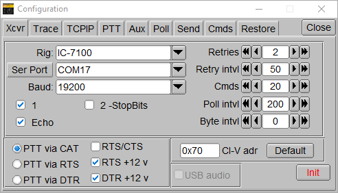
Here are my settings to get it working.
But for this post, I'm setting up OmniRig v2.1.
Categories covered here are:
OmniRig can be downloaded here.
So looking at the above flrig configuration, we can decern a few things.
The Xiegu Radio shares the same serial protocol as some Icom radios(IC-756-Pro and IC-7100).
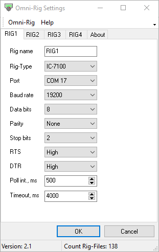
We will be using the IC-7100 Rig-Type.
We fire up WSJT-X and configure our radio settings as such.
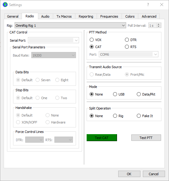
Now we are ready to test some WSPR signals :)
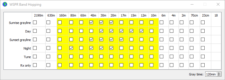
As I am using an end-fed antenna, it resonates at a few frequencies, and my band hopping schedule is set up as such.
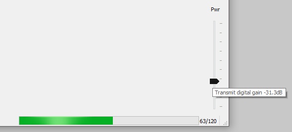
We set the power level on the radio to 2W.

Now we need to adjust the PWR in WSJT-X so that the ALC on the radio is around "098".

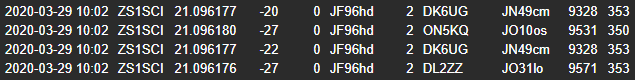
Here are the results from this transmission :)
Likewise, we would configure our input pwr for WSJT-X for all modes and frequencies :)

I hope this sheds some light on the usefulness of OmniRig.
No need to open anything once configured, just fire up WSJT-X and Enable Tx.
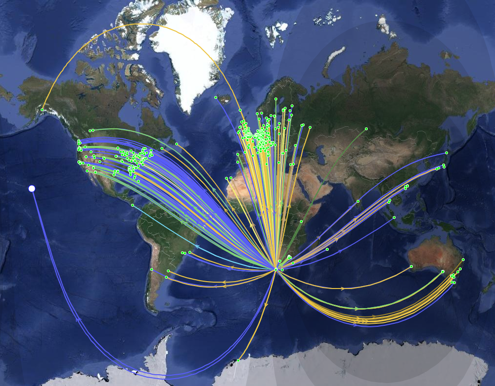
Here is an example of my performance over the past two weeks on 80-12m bands at 33dBm on WSPR.
Xiegu G90 and WSPR running 24/7.
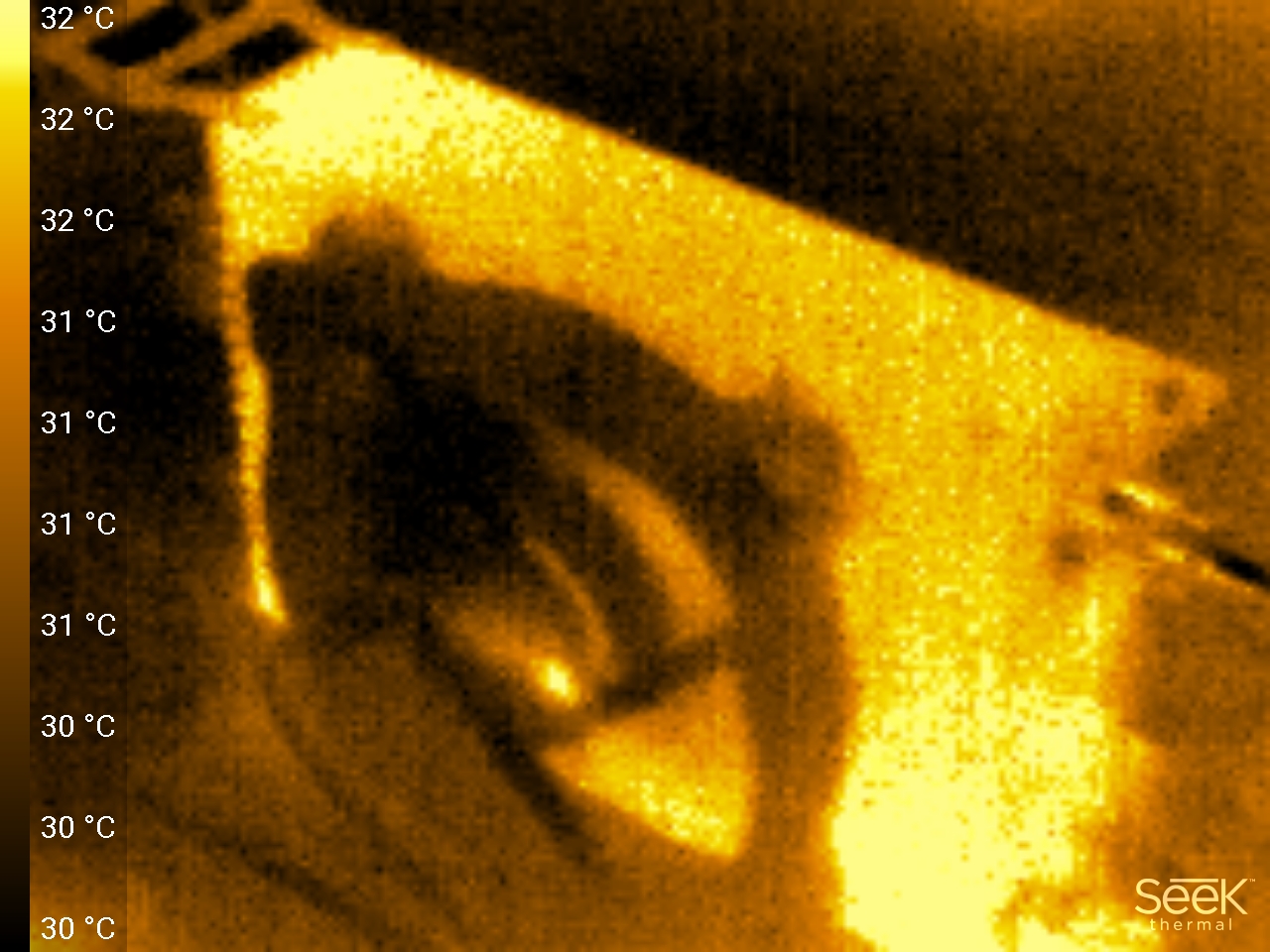
This required some form of cooling for the radio to run this long.
I used a 120mm computer chassis fan and some butyl tape to absorb the vibrations it might create.

It is connected in parallel to the radio's DC-IN.

It's optional but seems to do the job.
Right now that digital modes are out of the way, how about an I/Q pan-adapter for the G90?
Want to see more than just what is on the radio screen?
This is where we fire up HDSDR and configure it:
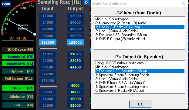
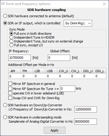
RF Front-End Configuration
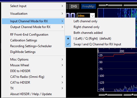
And you should be presented with a nice panoramic view of the RF spectrum, demodulation control as well as CAT Control.
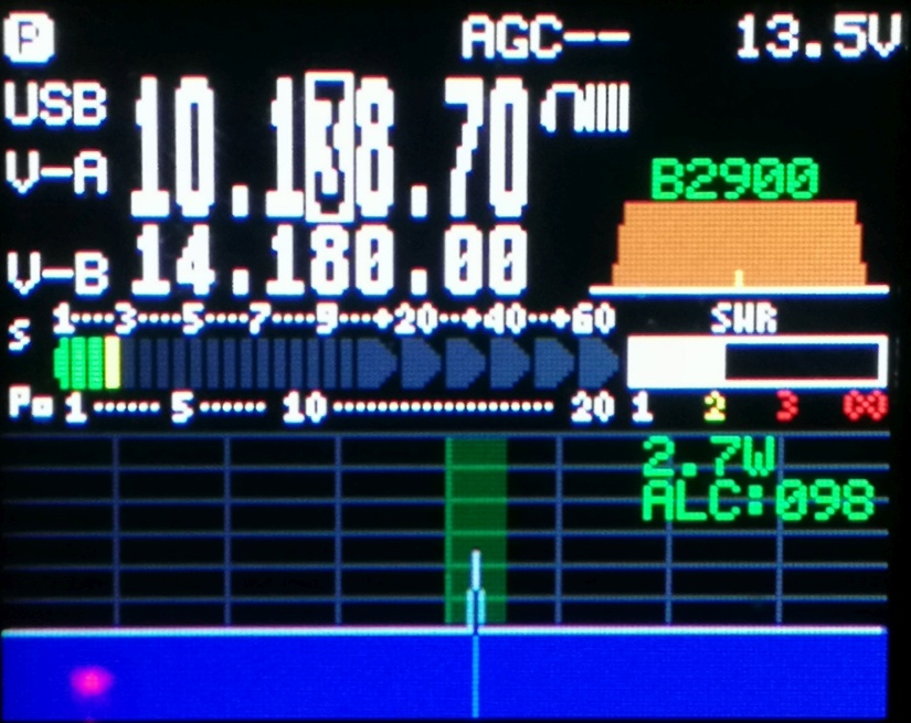
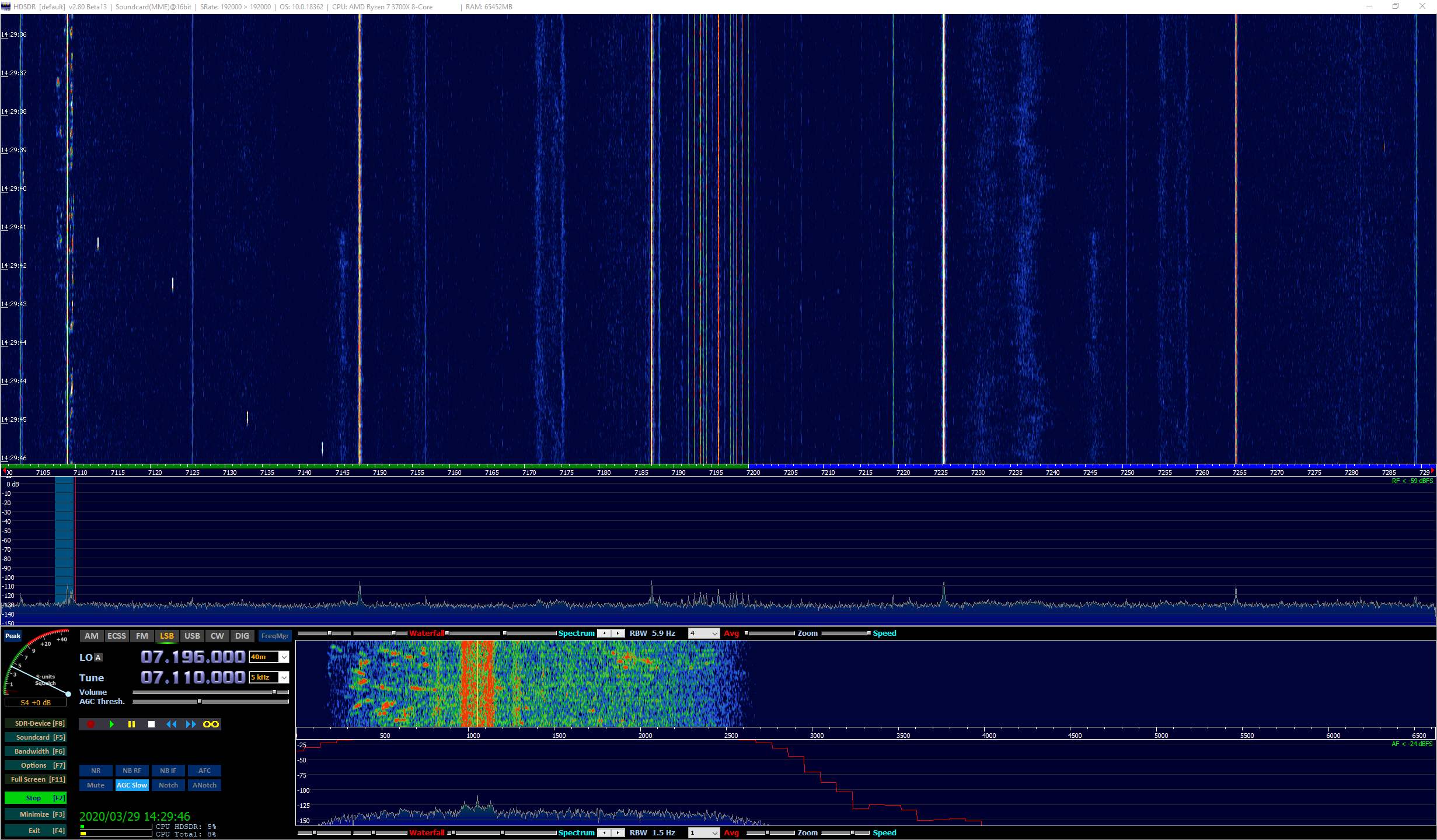
Here is 192kHz of goodness with a calibrated S-Meter :D
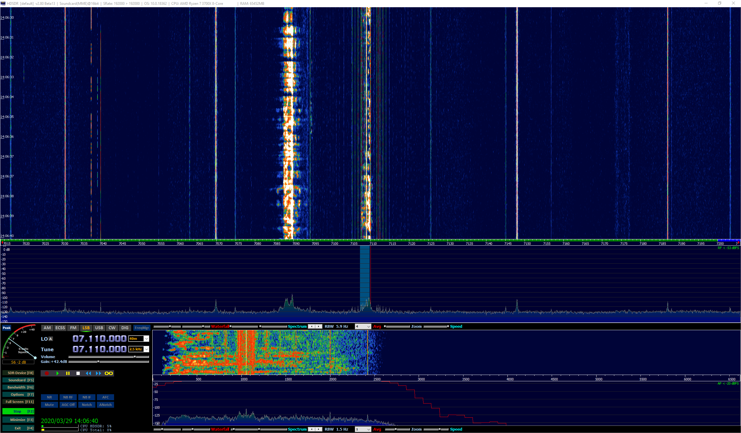
Here I am tuned to 7.196MHz on the radio, yet I am listening and seeing the spectrum on 7.110MHz

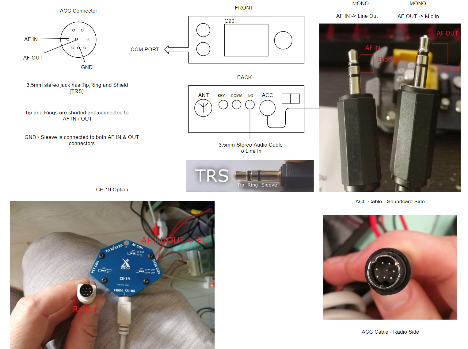
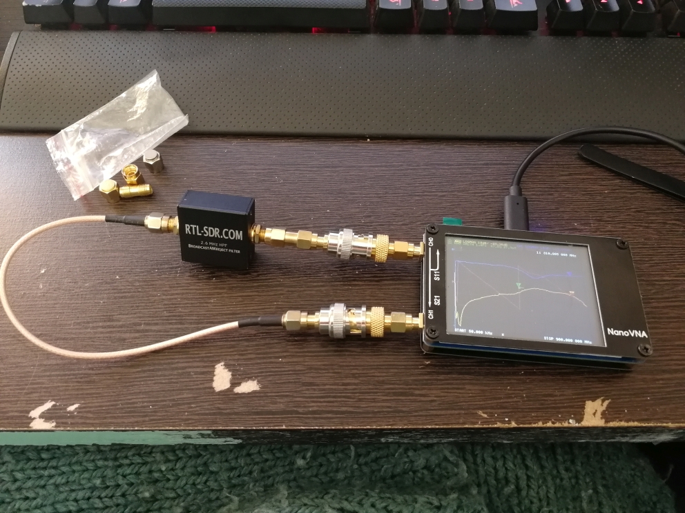
Wiring and setup pics requested.
I keep time with a USB Serial device and GPS
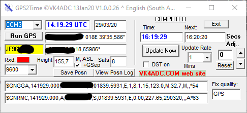
The actual GPS device L76X GPS module

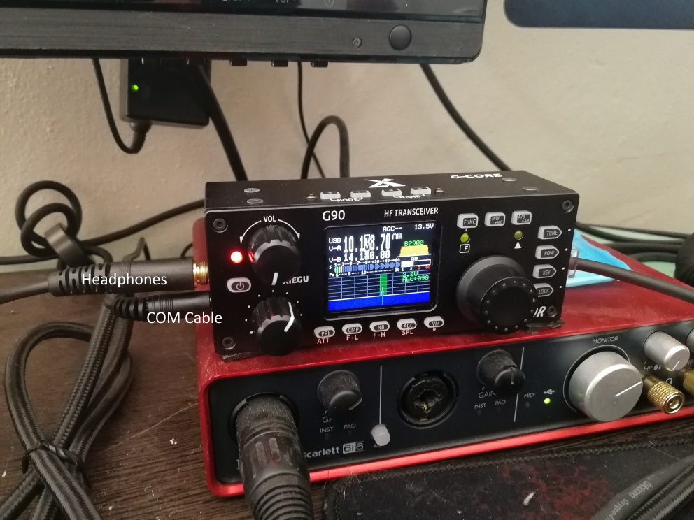

Communication is done with the Xiegu "programming" / CAT control cable that comes with the kit.
As can be seen, this radio is a competent little device, especially when properly set up.
I have a suspicion that some of these configurations should work with the Xiegu X5105 too.
Huzzah!
Kind Regards
Ohan
Hi
As I am naturally curious about RF Tech, I tend to collect devices that quantify certain aspects of the RF hobby.
This device is, by far been the most interesting one.
Some time ago, I wrote morfeusQt, which is still somewhat active...
So I contemplated writing a similar python application for this device.
Fortunately, I was searching GitHub for "nanovna" one night and this popped up.
It was Python, and it worked on first load and omg...
It's opensource!
It is written by Rune B. Broberg / 5Q5R.
In the following blog post will go through some vigorous screenshotting and brief texting to explain my process,
please bear with me as I run through its use cases, some of which I will cover in the next article as my understanding
on the matter deepens.
The steps that follow are:
I will forego going through the software repository cloning process and jump straight to usage.
This should yield the most satisfying results from this little USB serial device.
Please follow this link for the latest release page.
Once downloaded, let's have our nanoVNA device plugged in via the USB cable before firing up the application.
Once opened, we have a screen that looks like this.
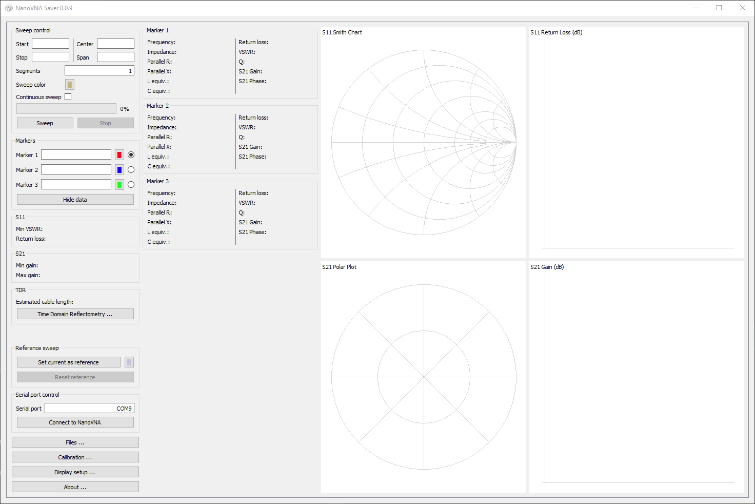
We then click on Connect to NanoVNA to initiate our device and get the first scan.
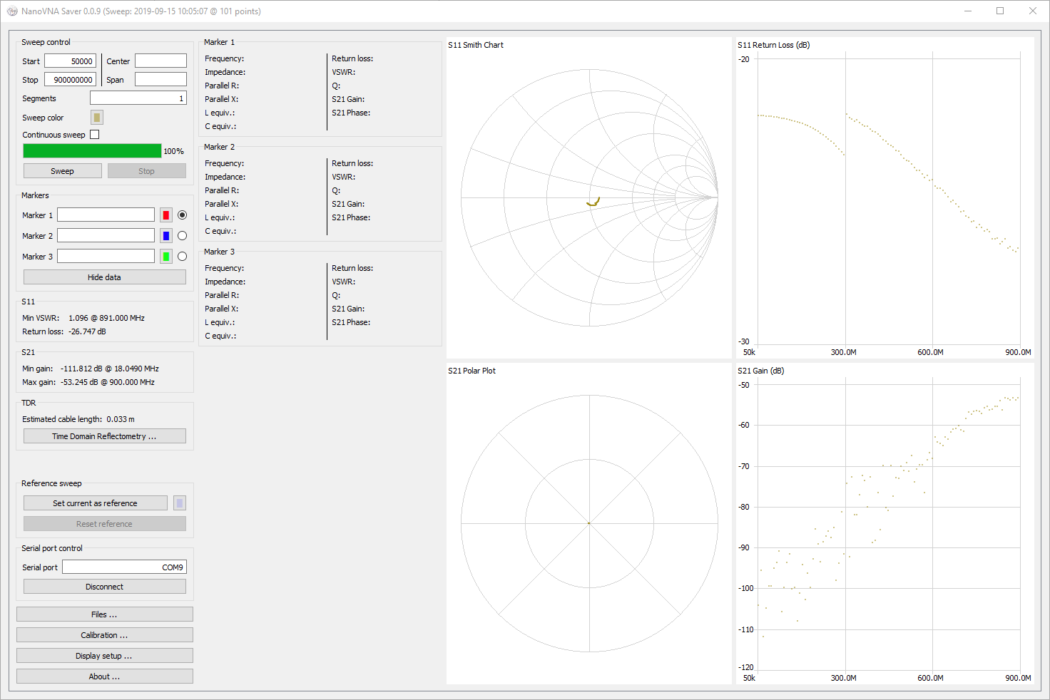
Here we are presented with a beautiful presentation of our data.
I am going to customise this display, and I do this by clicking on Display Setup and by changing the Sweep Color.
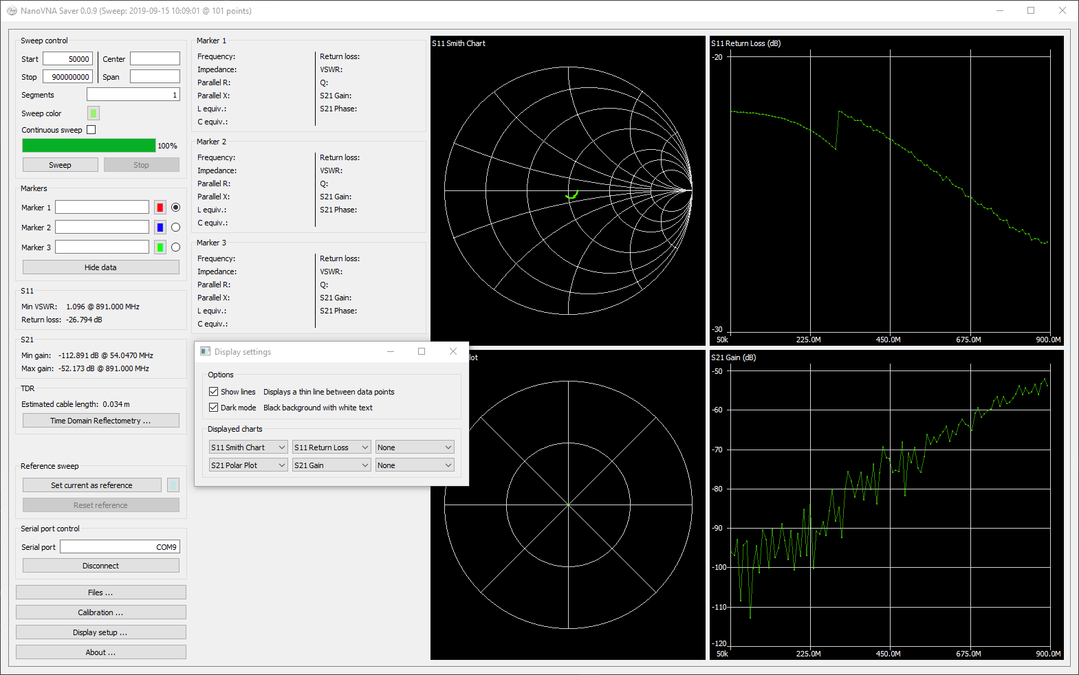
That's a little better...
Short
| Open
| Load
|
Through
| Isolation 2x 50Ω dummy loads
|
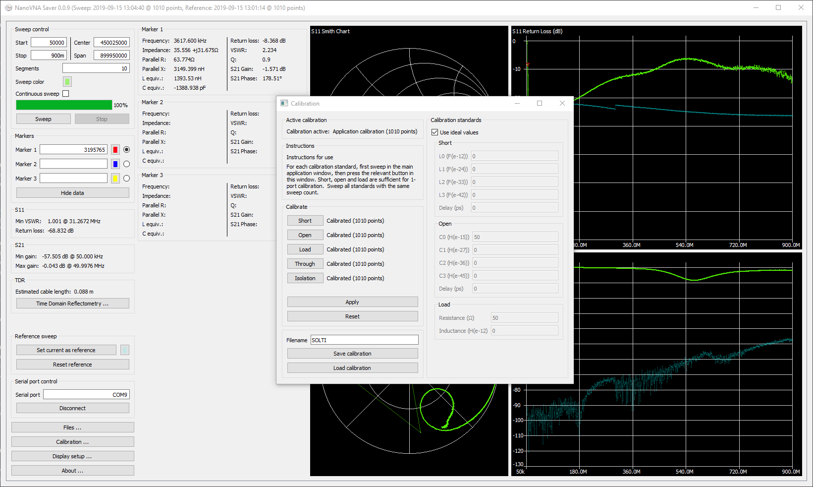
We click on calibration, and then we set our segments to 10 to have more points, after which we click sweep.
Once the sweep completes with our Short in place, we click the "short" button in the calibration screen.
Then after the OSL calibration is complete, we can click apply and then if we'd want we can save the calibration for later loading.
We then close our calibration screen.
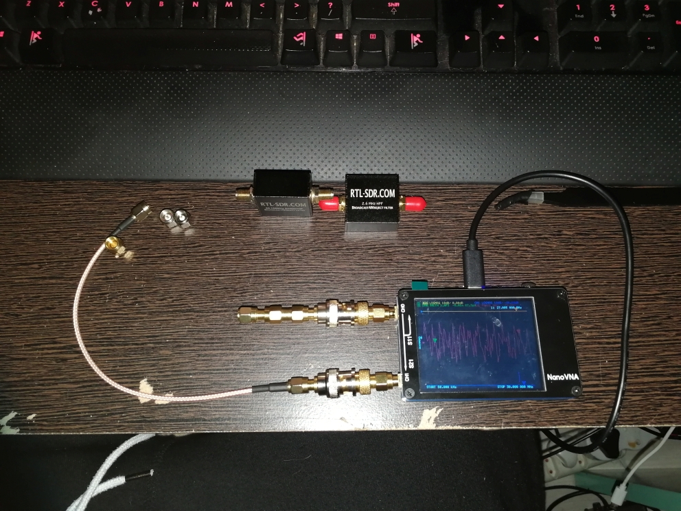
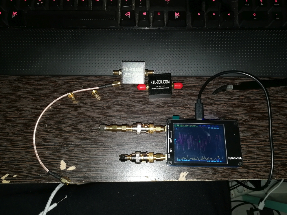
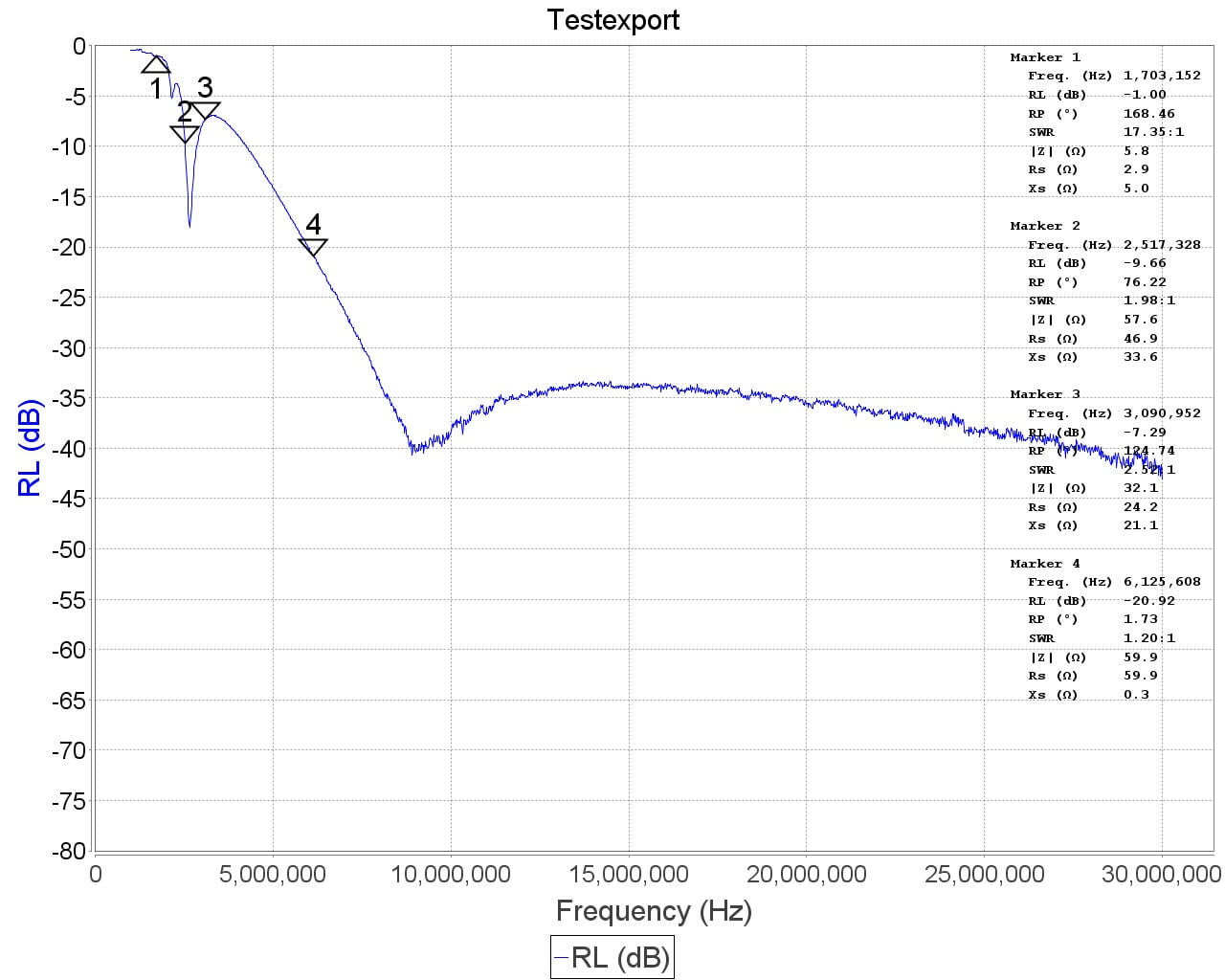
First up a 2.6MHz HPF from RTL-SDR.
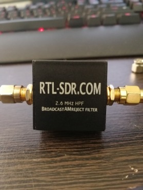 |  |
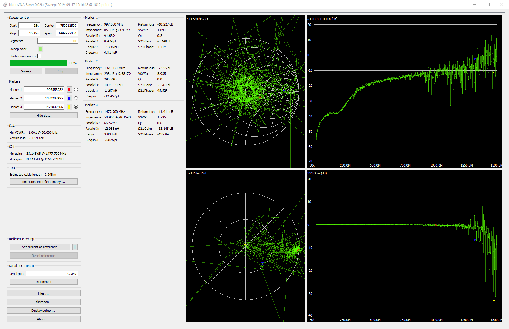
We sweep from 50KHz - 30MHz with ten segments for some excellent resolution(1010 data points)
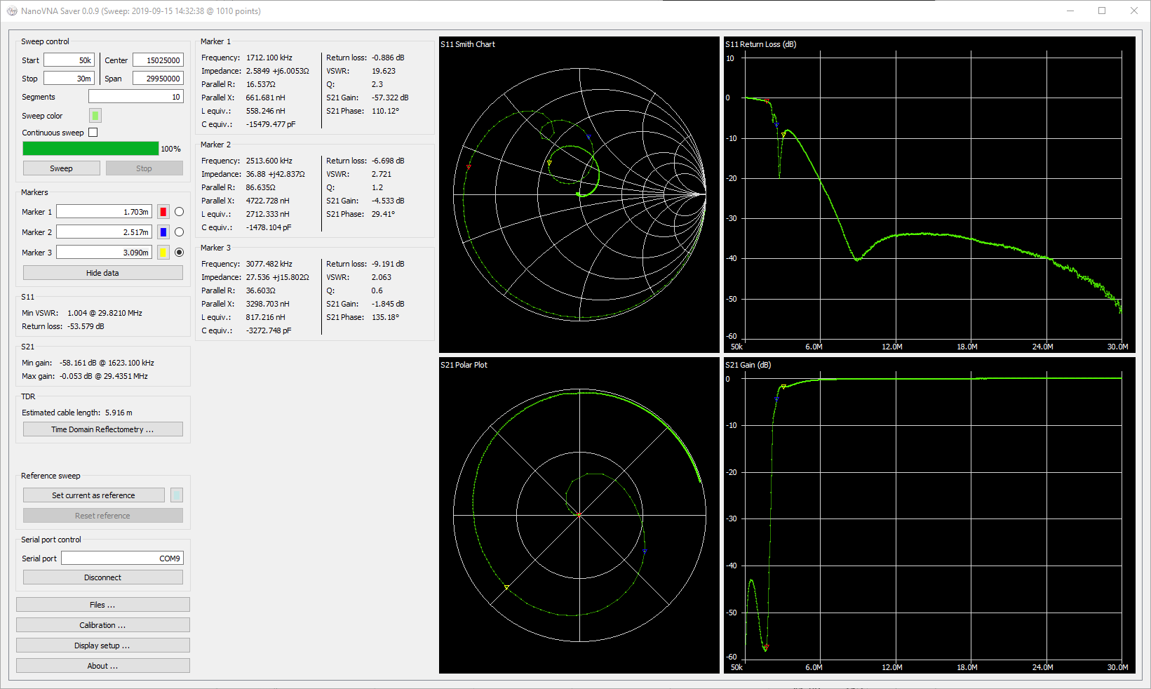
I've also added three markers to peak at values, to match the first markers in the chart below.
Markers points can be highlighted by selecting the appropriate radio box in the markers section.
It matches nicely with what s found on the RTL-SDR website
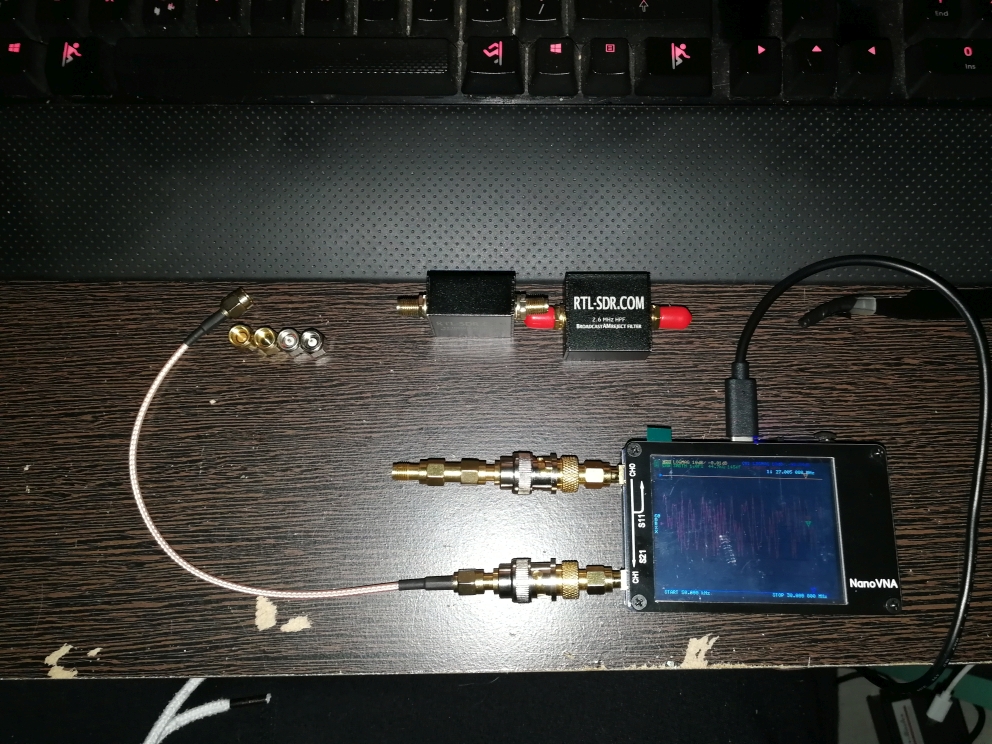
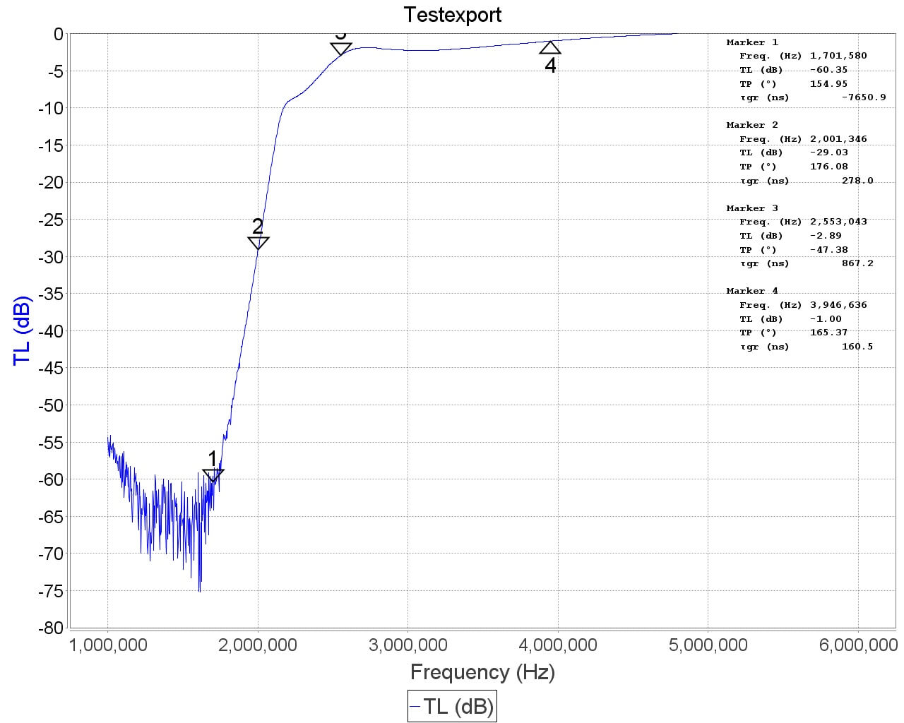
Next, we sweep from 50KHz-6MHz, for a closer look
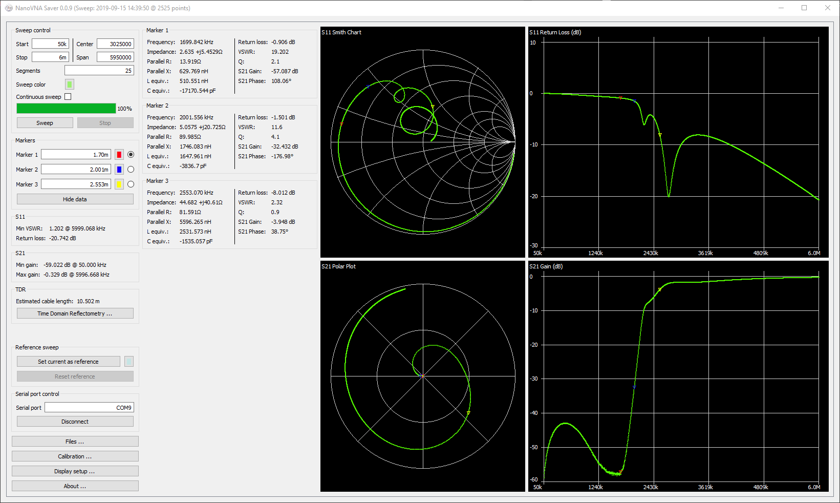
It also pairs nicely with what is on RTL-SDR
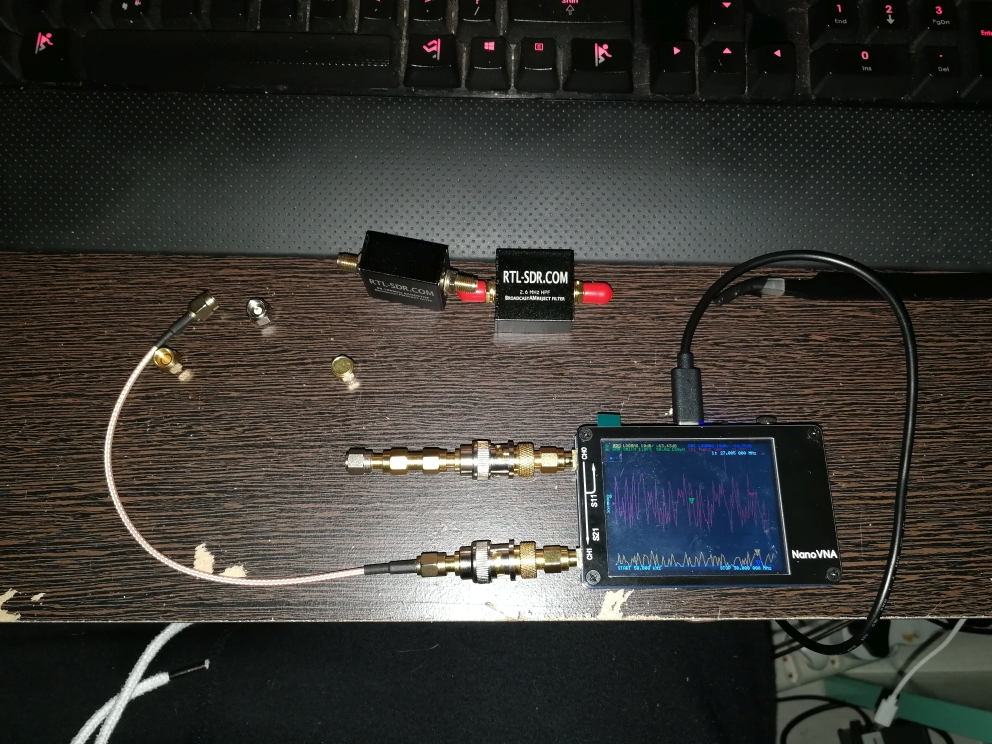
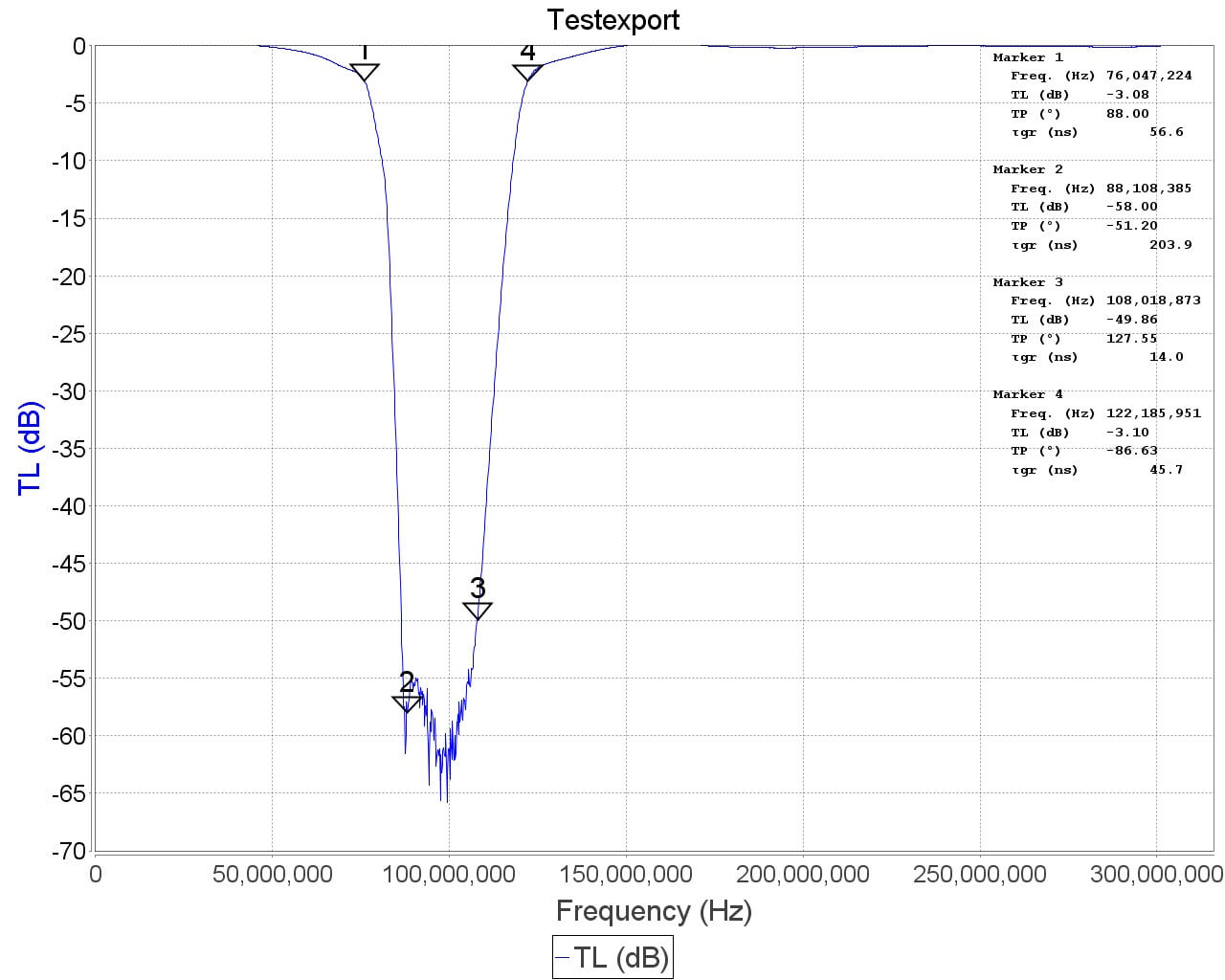
The 88-108MHz bandstop filter
 | 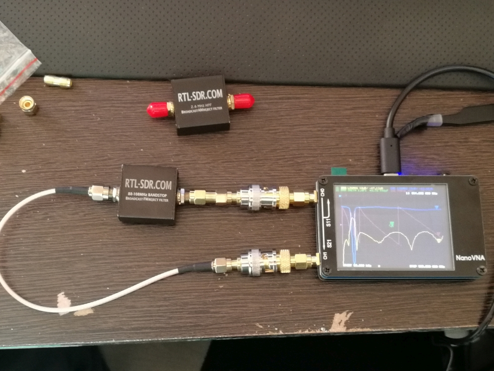 |
We sweep from 50KHz-300MHz
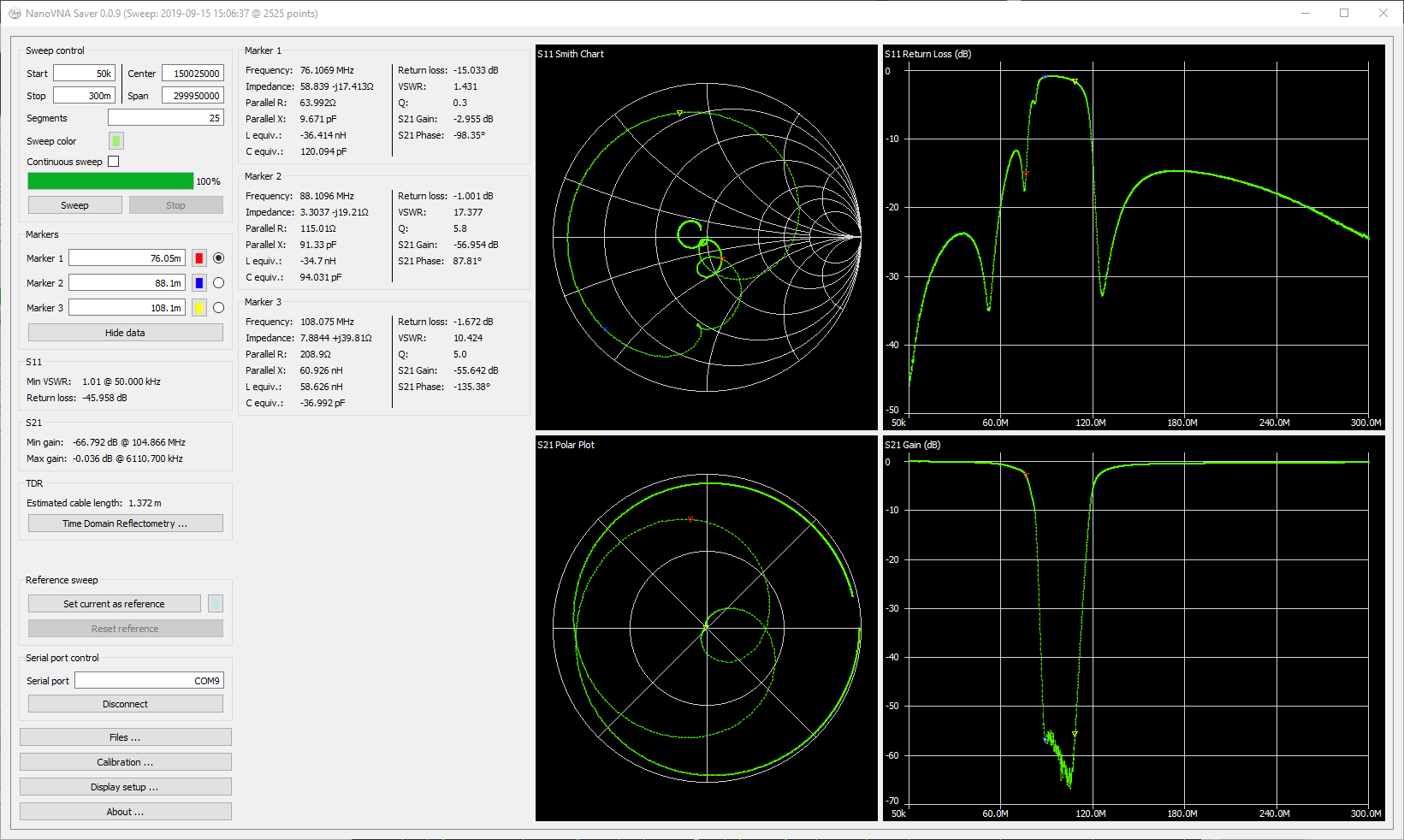
Again this matches quite nicely with what is on RTL-SDR
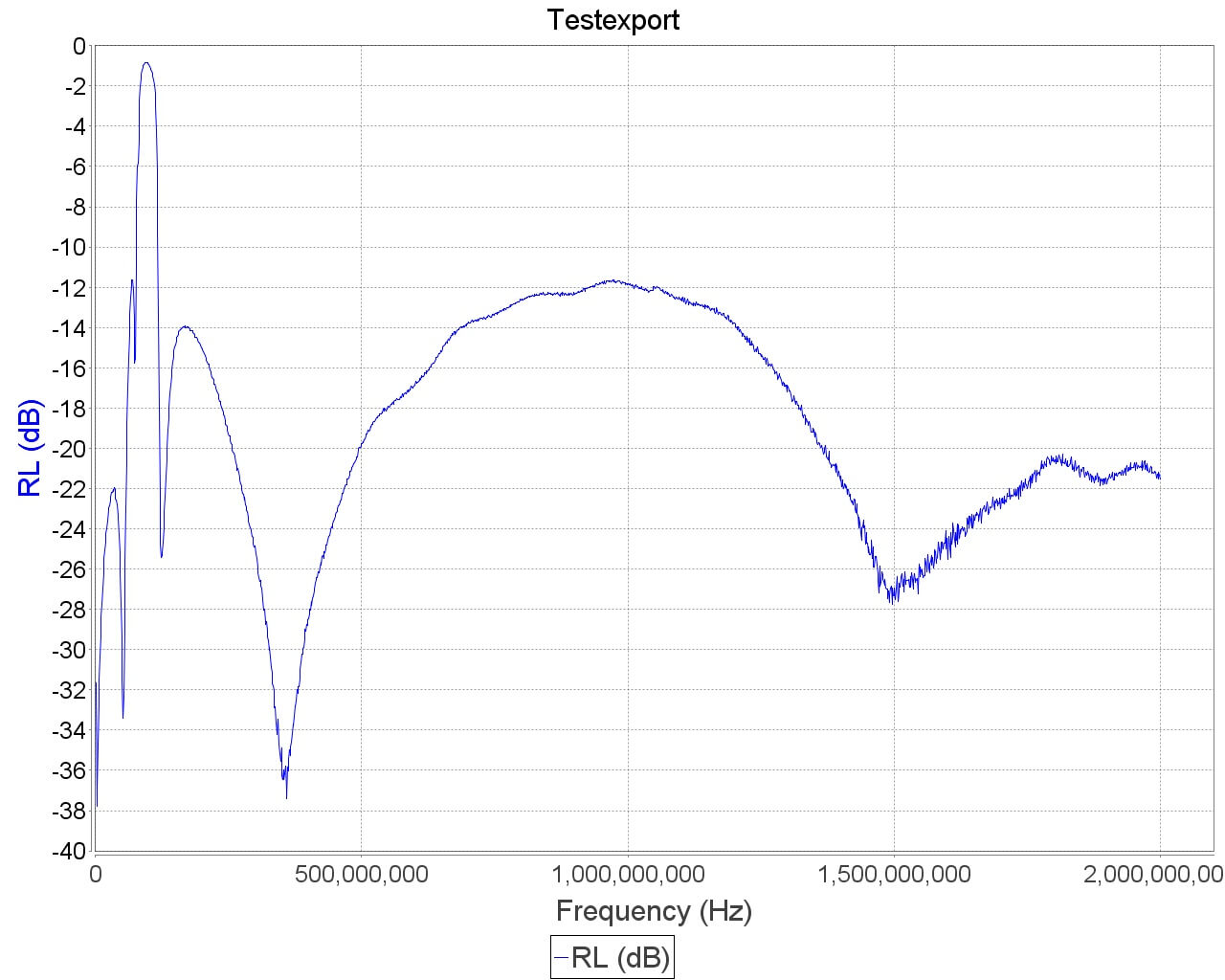
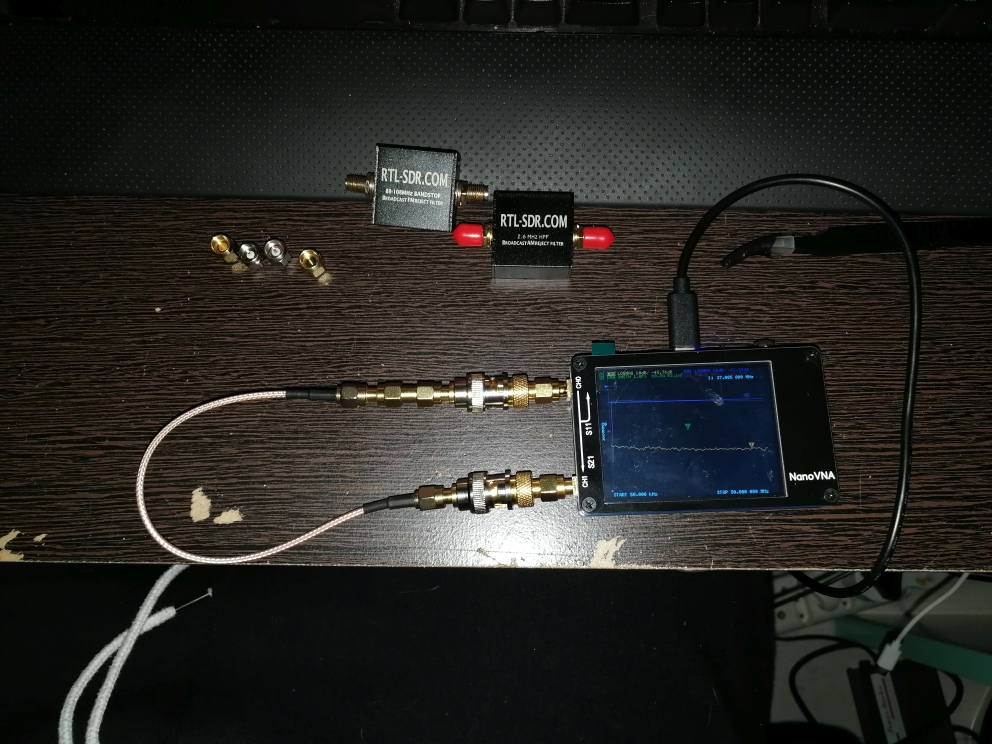
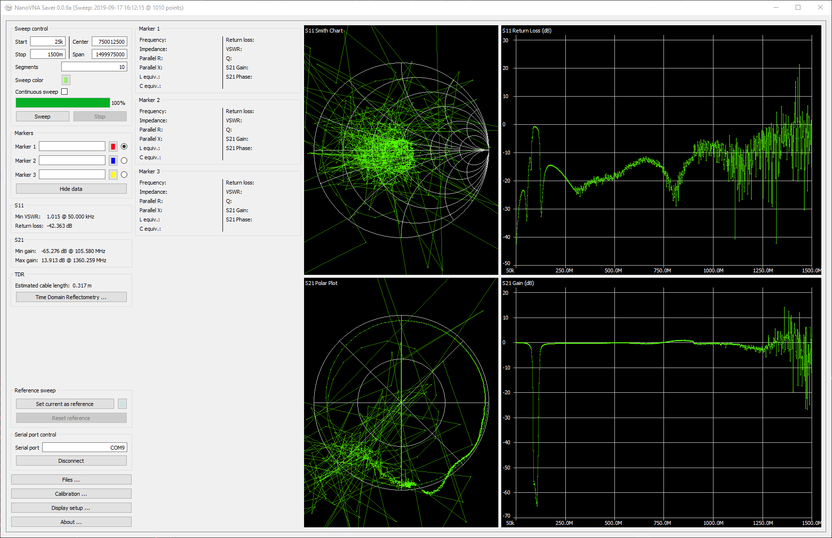
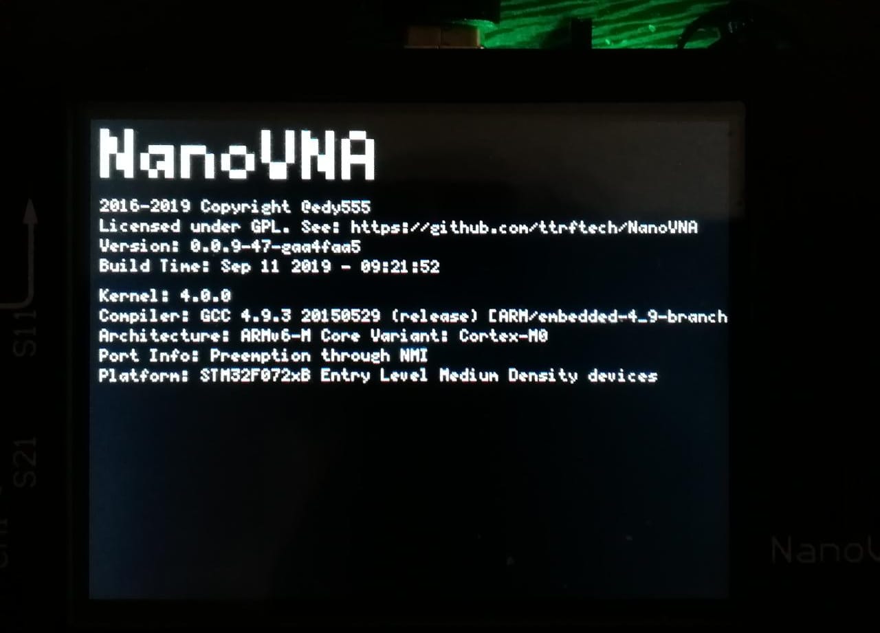
Here I tested a new master branch firmware update which expands the frequency range by 600MHz to 1.5GHz.
Here are some device captures with a 50Ω load


DFU can be entered via software switch

As can be seen below, the hardware limitations of the device are being met above 900MHz.
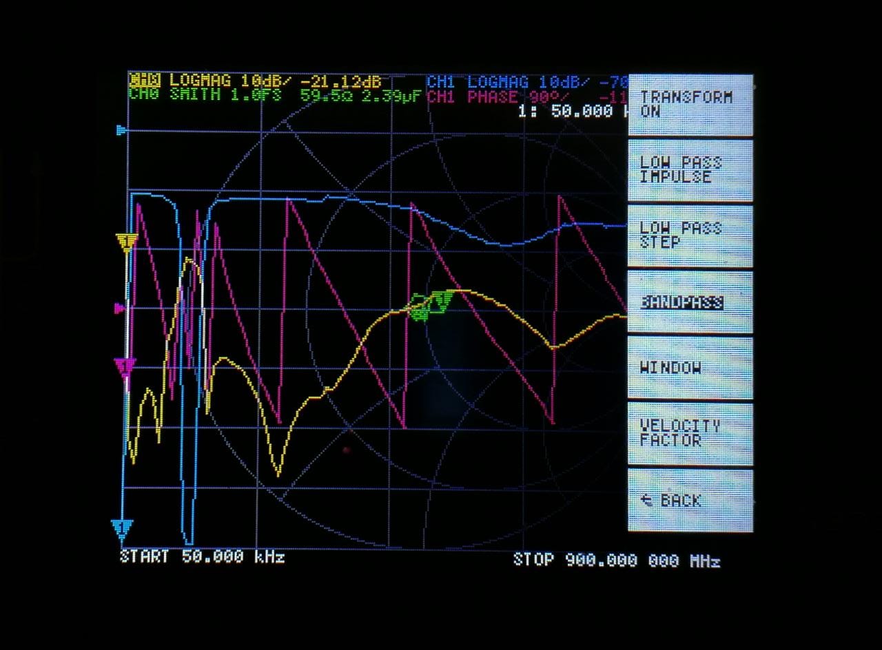
This is a sweep of the bandstop filter in place with a new calibration made for the new range in the latest firmware.
Here is the Open sweep with extended range
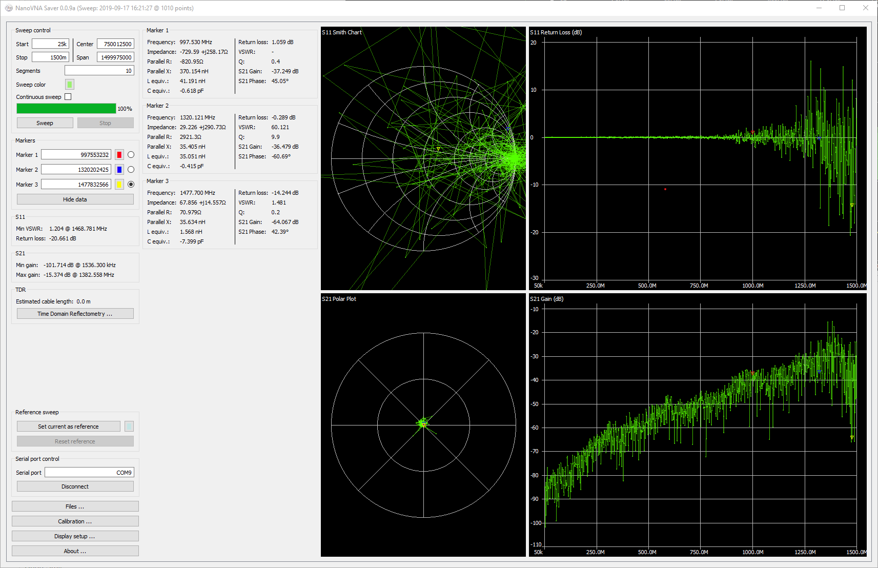
Here is the Short sweep with extended range
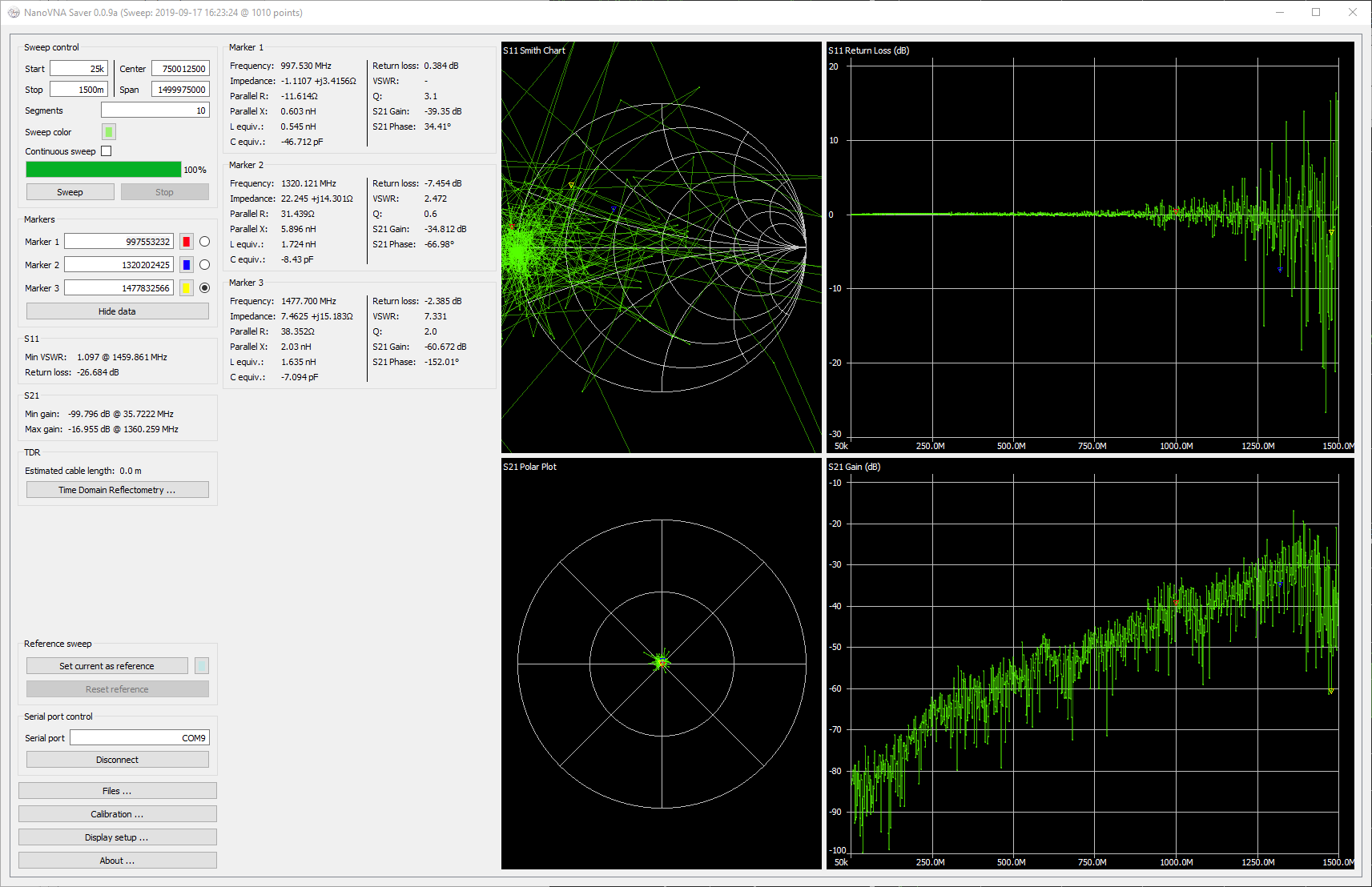
Here is the Load sweep with extended range
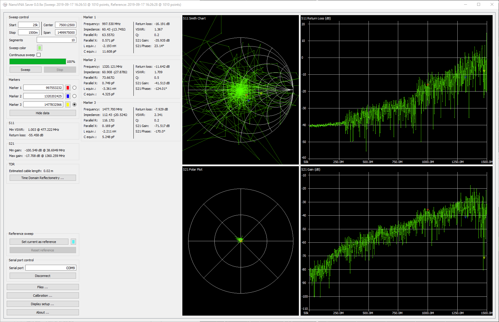
Here is the through sweep with extended range
Perhaps the device would need a hardware upgrade shortly?
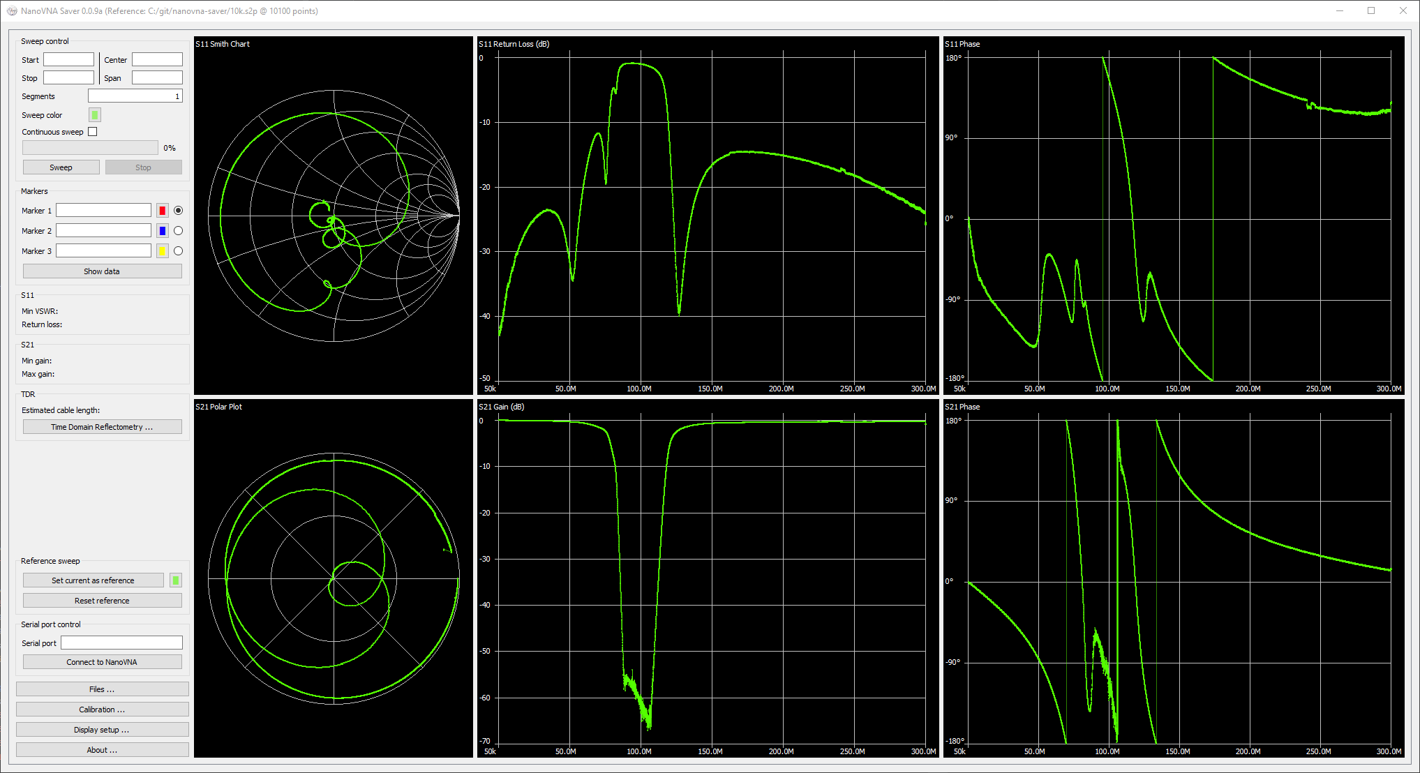
Just for science, how would it look with 10k points?
A sweep of 10100 points with the bandstop in place
:)
So for me being a radio amateur and loving building things, it's nice having a device that can quantify specific theoretical parameters.
I am also still learning a bunch, so much so that I decided to contribute to the GitHub project.
It is lovely to see the application grow with every iteration and Rune is definitely on the fast track to making
one of the most top-notch VNA applications for this device.
I would also like to thank the author of this article and Rune for pointing it out, it always great learner things from others in the same domain.
I'll get to measuring some antennas on the next Part, for now, if you'd be interested here
are some build instructions for the firmware in Ubuntu 19.04
Kind Regards
Ohan Smit
ZS1SCI
Hi
This will be a guide to building the NanoVNA source code from a fresh Ubuntu machine.
sudo apt-get install git
ssh-keygen -t rsa -b 4096 -C "your_email@domain.com"
eval "$(ssh-agent -s)"
ssh-add ~/.ssh/id_rsa
sudo apt-get install xclip
xclip -sel clip < ~/.ssh/id_rsa.pub
Click the green New SSH Key button

Give it a Title and paste the copied key in this window

wget https://developer.arm.com/-/media/Files/downloads/gnu-rm/8-2018q4/gcc-arm-none-eabi-8-2018-q4-major-linux.tar.bz2
sudo tar xfj gcc-arm-none-eabi-8-2018-q4-major-linux.tar.bz2 -C /usr/local
PATH=/usr/local/gcc-arm-none-eabi-8-2018-q4-major/bin:$PATH
sudo apt install -y dfu-util
git clone https://github.com/ttrftech/NanoVNA.git && cd NanoVNA
git submodule update --init --recursive

Type yes when asked
If you see something like this
Submodule path 'ChibiOS': checked out '669d4bbc8da1ee0e4ccdf93a472b06d183922320'
All is good!!!
make

That's a successful build right there!
Update :
Short the two pins in the red circle with the device powered off, then with the pins shorted power on the device.
This will enter DFU mode, with a blank white screen.
The device can now be flashed.

Software Reset to DFU

make flash

This is what to expect when flashing the device.
For conversion to dfuse dfu file format for Windows flashers:
In the ubuntu terminal still:
dfu-tool convert dfuse ./build/ch.hex test.dfu
Set PID, VID:
dfu-tool set-product test.dfu df11
dfu-tool set-vendor test.dfu 0483

Experimental build from a branch that enables Time Domain Stuff
Added menu items
Hopefully, this will help some folks get to building the firmware of this device.
Kind Regards
Ohan
ZS1SCI
I recently bought a NanoVNA of amazon following the article on RTL-SDR.
Yes, I got the bad model, no shielding, no QC, I had to fix the short to GND on the USB-C header, but after getting it working, its a very nifty tool for the RF shack.
My friend ZS1ARB told me about this article written by Salil aka nuclearrambo.
It goes into detail on how to calculate the length of a cable using the NanoVNA as a Time-domain reflectometer.
This animation explains it rather elegantly.
![]()
I highly recommend you start there.
This blog would just to show how I used this technique to measure the length of coax cable rather accurately.
Here he provides us with a Python script for calculating the distance of a given coax cable. I've modified his original a bit.
import skrf as rf
import matplotlib.pyplot as plt
from scipy import constants
import numpy as np
import sys

raw_points = 101
NFFT = 16384
PROPAGATION_SPEED = 78.6 #For RG58U
plt_filename = sys.argv[1]
_prop_speed = PROPAGATION_SPEED/100
cable = rf.Network(plt_filename)
print(plt_data)
 #Read skrf docs
print(cable)
s11 = cable.s[:, 0, 0]
print(type(s11))
window = np.blackman(raw_points)
s11 = window * s11
td = np.abs(np.fft.ifft(s11, NFFT))
#print(s11)

#Calculate maximum time axis
t_axis = np.linspace(0, 1/cable.frequency.step, NFFT)
d_axis = constants.speed_of_light * _prop_speed * t_axis

#find the peak and distance
pk = np.max(td)
idx_pk = np.where(td == pk)[0]
cable_len  = d_axis[idx_pk[0]]/2
#print(cable_len)
#print(d_axis)
# Plot time response

plt.plot(d_axis, td)
plt.xlabel("Distance (m) Length of cable(%.5fm)" % cable_len)
plt.ylabel("Magnitude")
plt.title("Return loss Time domain")
plt.show()
Instead of saving a file, running a python script and then only seeing this script's results, I decided to glue these two together for the time being.
I modified some parameters for my use. Here I just took the filename and sent that path to the python script.
plt_filename = sys.argv[1]
cable = rf.Network(plt_filename)
I also happen to find that Roger Clark had also conveniently reverse engineered the windows C# app for NanoVNASharp that's on the email groups.
So I cloned his repo, added some C# code to make the Python script run.
If you'd like to make this run.
Here you would have to change the python path in the below code
...
psi.FileName = @"YOUR FULL PATH HERE";
...
var script = @"CLONED DIR PATH\tdr.py";
...
and the script location to the cloned repository directory path it should look something like this.
 public void RunPython(string filename)
 {
            var psi = new ProcessStartInfo();
            psi.FileName = @"C:\Users\SomeUser\AppData\Local\Programs\Python\Python36\python.exe";
            var script = @"C:\NanoVNASharp\tdr.py";
            psi.Arguments = $"\"{script}\" \"{filename}\"";
            psi.UseShellExecute = false;
            psi.CreateNoWindow = true;
            psi.RedirectStandardOutput = true;
            psi.RedirectStandardError = true;
            var errors = "";
            using (var process = Process.Start(psi))
            {
                errors = process.StandardError.ReadToEnd();

            }
            Console.WriteLine("ERRORS");
            Console.WriteLine(errors);
}
and voila now when you save the s1p file in NanoVNASharp it will open the python script after the save dialogbox has been closed.
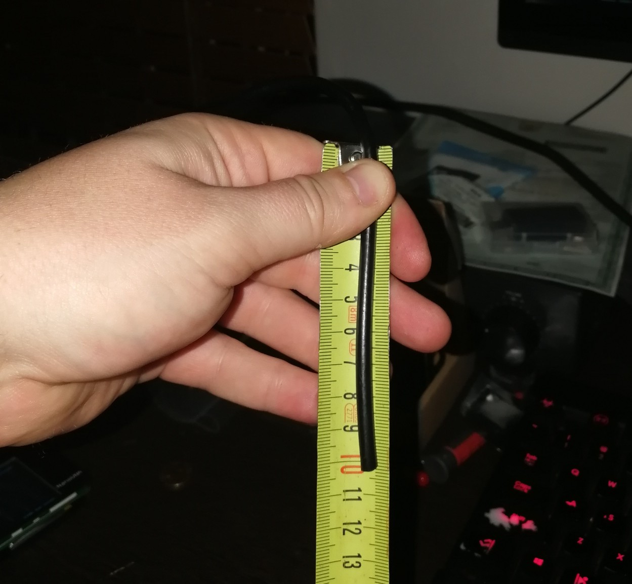
So my first course of action for getting the Velocity factor of the cable I was measuring was to physically measure the cable first.
It came out to 4645 mm, excellent now let's try some various velocities on line 8 the Python script and see what we get.
Velocity: 75% and Length calculated: 4432 mm, not quite what we want.
Velocity: 79% and Length calculated: 4669 mm, mmmh to much hey...
Eventually, it came to a velocity factor of 78.6% with a calculated distance of 4645.71mm
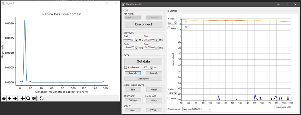
So I cut off a piece of wire about 10cm in length.
I then pressed the Get Data button clicked Save s1p, gave it a file name and then was presented with a pretty cool finding XD
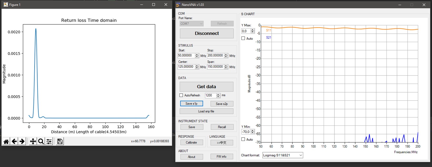
4545.03mm XD that is pretty neat!
I will see if how far I'd take this reverse-engineered project, for now, this was just an informatory post.
Might have to build some other interface to add a few things.
This is me sharing my discovery.
ZS1SCI